On June 25th, 2020, the first official version of YOLOv5 was released by Ultralytics, a computer vision model used for detecting objects.
In this article we hope to address some of the following questions about YOLOv5:
- What's new in YOLO v5?
- How does YOLO v5 compare to YOLO v4?
- What's different between YOLO v4 and YOLO v5?
- Should I use YOLO v4 or YOLO v5 for object detection?
Let's begin!
What is YOLOv5?
YOLOv5 is a model in the You Only Look Once (YOLO) family of computer vision models. YOLOv5 is commonly used for detecting objects. YOLOv5 comes in four main versions: small (s), medium (m), large (l), and extra large (x), each offering progressively higher accuracy rates. Each variant also takes a different amount of time to train.
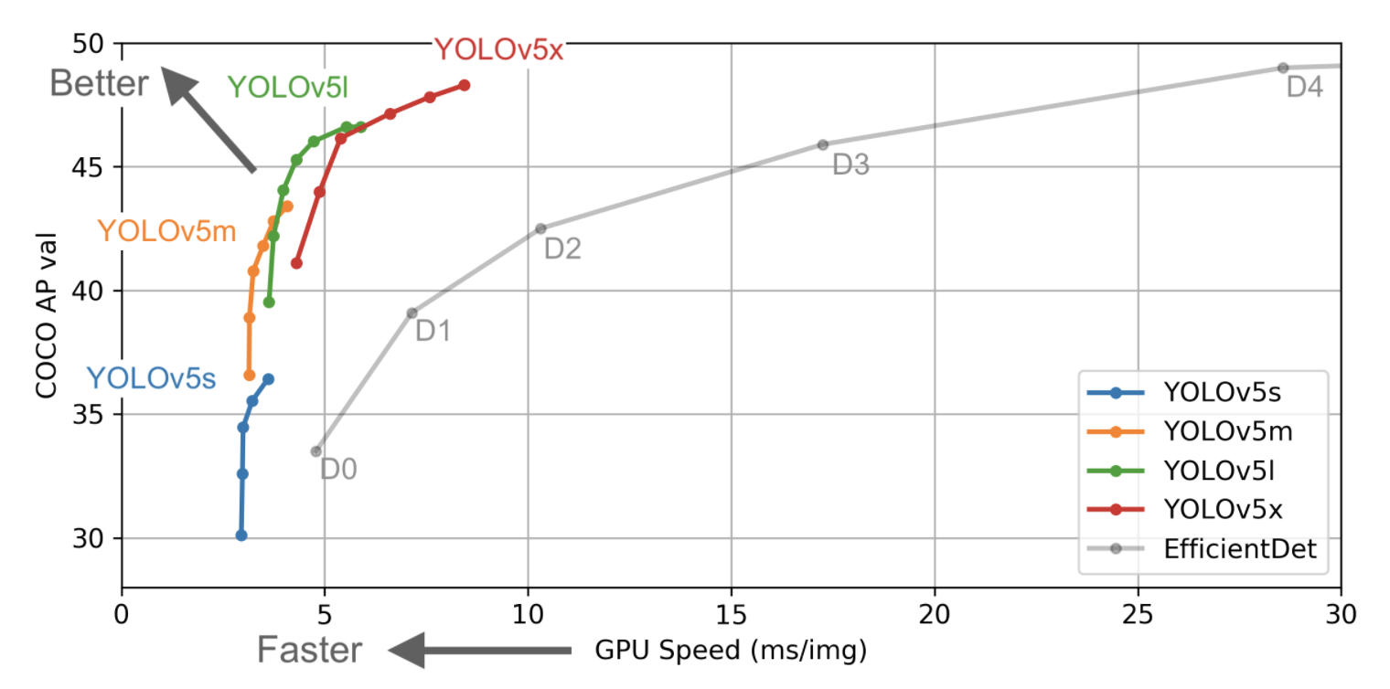
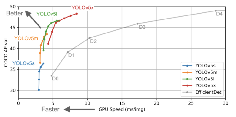
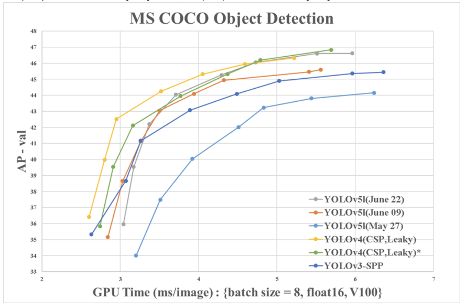
In the chart, the goal is to produce an object detector model that is very performant (Y-axis) relative to it's inference time (X-axis). Preliminary results show that YOLOv5 does exceedingly well to this end relative to other state of the art techniques.
In the chart above, you can see that all variants of YOLOv5 train faster than EfficientDet. The most accurate YOLOv5 model, YOLOv5x, can process images multiple times faster with a similar degree of accuracy than the EfficientDet D4 model. This data is discussed in more depth later in the post.
YOLOv5 derives most of its performance improvement from PyTorch training procedures, while the model architecture remains close to YOLOv4.
Looking to train a custom model?
Skip this post and jump straight to our YOLOv5 tutorial. You'll have a trained YOLOv5 model on your custom data in minutes.
A short interview with the creator of YOLOv5. Subscribe to our YouTube channel for more.
Origin of YOLOv5: An Extension of YOLOv3 PyTorch
The YOLOv5 repository is a natural extension of the YOLOv3 PyTorch repository by Glenn Jocher. The YOLOv3 PyTorch repository was a popular destination for developers to port YOLOv3 Darknet weights to PyTorch and then move forward to production. Many (including our vision team at Roboflow) liked the ease of use the PyTorch branch and would use this outlet for deployment.
After fully replicating the model architecture and training procedure of YOLOv3, Ultralytics began to make research improvements alongside repository design changes with the goal of empowering thousands of developers to train and deploy their own custom object detectors to detect any object in the world. This is a goal we share here at Roboflow.
The following image shows some of the updates that were made by Ultralytics:
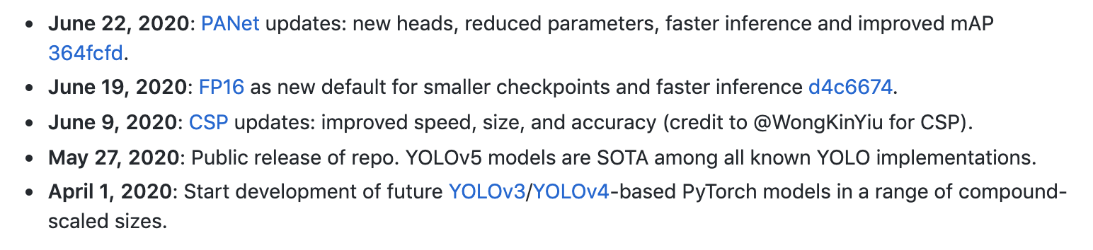
These advancements were originally termed YOLOv4 due to the recent release of YOLOv4 in the Darknet framework, the model was renamed to YOLOv5 to avoid version collisions. There was quite a bit of debate around the YOLOv5 naming in the beginning and we published an article comparing YOLOv4 and YOLOv5, where you can run both models side by side on your own data.
We abstain from custom dataset comparisons in this article and just discuss the new technologies and metrics that the YOLO researchers are publishing on GitHub discussions.
It is worth noting, since the repository was published, significant research progress has occurred in YOLOv5, which we expect to continue, and might give some justification to the YOLO-"moniker". Thus, YOLOv5 is by no means a finished model: it will evolve over time.
An Overview of the YOLOv5 Architecture
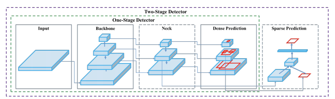
Object detection, a use case for which YOLOv5 is designed, involves creating features from input images. These features are then fed through a prediction system to draw boxes around objects and predict their classes.
The YOLO model was the first object detector to connect the procedure of predicting bounding boxes with class labels in an end to end differentiable network.
The YOLO network consists of three main pieces.
- Backbone: A convolutional neural network that aggregates and forms image features at different granularities.
- Neck: A series of layers to mix and combine image features to pass them forward to prediction.
- Head: Consumes features from the neck and takes box and class prediction steps.
With that said, there are many approaches one can take to combining different architectures at each major component. The contributions of YOLOv4 and YOLOv5 are foremost to integrate breakthroughs in other areas of computer vision and prove that as a collection, they improve YOLO object detection.
An Overview of YOLO Training Procedures
The procedures taken to train a model are just as important as any factor to the end performance of an object detection system, although they are often less discussed. Let's talk about two main training procedures in YOLOv5:
- Data Augmentation: Data augmentation makes transformations to the base training data to expose the model to a wider range of semantic variation than the training set in isolation.
- Loss Calculations: YOLO calculates a total loss function from the GIoU, obj, and class losses functions. These functions can be carefully constructed to maximize the objective of mean average precision.
YOLOv5 for PyTorch
The largest contribution of YOLOv5 is to translate the Darknet research framework to the PyTorch framework. The Darknet framework is written primarily in C and offers fine grained control over the operations encoded into the network. In many ways the control of the lower level language is a boon to research, but it can make it slower to port in new research insights, as one writes custom gradient calculations with each new addition.
The process of translating (and exceeding) the training procedures in Darknet to PyTorch in YOLOv3 is no small feat.
Data Augmentation in YOLOv5
With each training batch, YOLOv5 passes training data through a data loader, which augments data online. The data loader makes three kinds of augmentations:
- Scaling.
- Color space adjustments.
- Mosaic augmentation.
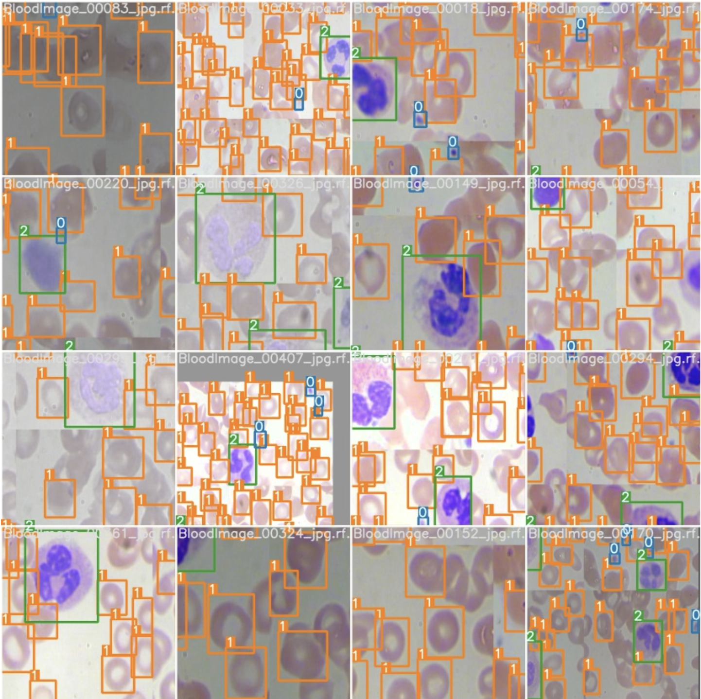
The most novel of these being mosaic data augmentation, which combines four images into four tiles of random ratio.
The mosaic data loader is native to the YOLOv3 PyTorch and now YOLOv5 repo.
Mosaic augmentation is especially useful for the popular COCO object detection benchmark, helping the model learn to address the well known "small object problem" - where small objects are not as accurately detected as larger objects.
It is worth noting that it worth experimenting with your own series of augmentations to maximize performance on your custom task.
Here is a picture of augmented training images in YOLOv5:
For a deep dive on how data augmentation has improved object detection models, I recommend reading this post on data augmentation in YOLOv4.
Auto Learning Bounding Box Anchors
In the YOLOv3 PyTorch repo, Glenn Jocher introduced the idea of learning anchor boxes based on the distribution of bounding boxes in the custom dataset with K-means and genetic learning algorithms. This is very important for custom tasks, because the distribution of bounding box sizes and locations may be dramatically different than the preset bounding box anchors in the COCO dataset.
In order to make box predictions, the YOLOv5 network predicts bounding boxes as deviations from a list of anchor box dimensions.
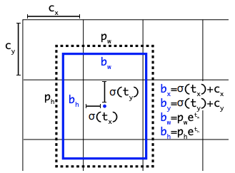
The most extreme difference in anchor boxes may occur if we are trying to detect something like giraffes that are very tall and skinny or manta rays that are very wide and flat. All YOLO anchor boxes are auto-learned in YOLOv5 when you input your custom data.
The following code illustrates an example of anchors that have been learned from training data in a YOLOv5 configuration file.
# parameters
nc: 80  # number of classes
depth_multiple: 0.33  # model depth multiple
width_multiple: 0.50  # layer channel multiple

# anchors
anchors:
  - [116,90, 156,198, 373,326]  # P5/32
  - [30,61, 62,45, 59,119]  # P4/16
  - [10,13, 16,30, 33,23]  # P3/8

# YOLOv5 backbone
The anchors in the YOLOv5 config file are now auto learned based on training data.
16 Bit Floating Point Precision
The PyTorch framework allows the ability to half the floating point precision in training and inference from 32 bit to 16 bit precision. When used with YOLOv5, this significantly speeds up the inference time of models.
However, the speed improvements are only available on select GPUs at this point - namely, V100 and T4. That said, NVIDIA has written intent to improve their coverage of this efficiency boost.
New Model Configuration Files
YOLOv5 formulates model configuration in .yaml, as opposed to the .cfg files used in Darknet. The main difference between these two formats is that the .yaml file is condensed to just specify the different layers in the network and then multiplies those by the number of layers in the block.
The new .yaml format looks like the following:
# parameters
nc: 80  # number of classes
depth_multiple: 0.33  # model depth multiple
width_multiple: 0.50  # layer channel multiple

# anchors
anchors:
  - [116,90, 156,198, 373,326]  # P5/32
  - [30,61, 62,45, 59,119]  # P4/16
  - [10,13, 16,30, 33,23]  # P3/8

# YOLOv5 backbone
backbone:
  # [from, number, module, args]
  [[-1, 1, Focus, [64, 3]],  # 0-P1/2
   [-1, 1, Conv, [128, 3, 2]],  # 1-P2/4
   [-1, 3, BottleneckCSP, [128]],
   [-1, 1, Conv, [256, 3, 2]],  # 3-P3/8
   [-1, 9, BottleneckCSP, [256]],
   [-1, 1, Conv, [512, 3, 2]],  # 5-P4/16
   [-1, 9, BottleneckCSP, [512]],
   [-1, 1, Conv, [1024, 3, 2]], # 7-P5/32
   [-1, 1, SPP, [1024, [5, 9, 13]]],
  ]

# YOLOv5 head
head:
  [[-1, 3, BottleneckCSP, [1024, False]],  # 9

   [-1, 1, Conv, [512, 1, 1]],
   [-1, 1, nn.Upsample, [None, 2, 'nearest']],
   [[-1, 6], 1, Concat, [1]],  # cat backbone P4
   [-1, 3, BottleneckCSP, [512, False]],  # 13

   [-1, 1, Conv, [256, 1, 1]],
   [-1, 1, nn.Upsample, [None, 2, 'nearest']],
   [[-1, 4], 1, Concat, [1]],  # cat backbone P3
   [-1, 3, BottleneckCSP, [256, False]],
   [-1, 1, nn.Conv2d, [na * (nc + 5), 1, 1]],  # 18 (P3/8-small)

   [-2, 1, Conv, [256, 3, 2]],
   [[-1, 14], 1, Concat, [1]],  # cat head P4
   [-1, 3, BottleneckCSP, [512, False]],
   [-1, 1, nn.Conv2d, [na * (nc + 5), 1, 1]],  # 22 (P4/16-medium)

   [-2, 1, Conv, [512, 3, 2]],
   [[-1, 10], 1, Concat, [1]],  # cat head P5
   [-1, 3, BottleneckCSP, [1024, False]],
   [-1, 1, nn.Conv2d, [na * (nc + 5), 1, 1]],  # 26 (P5/32-large)

   [[], 1, Detect, [nc, anchors]],  # Detect(P5, P4, P3)
  ]
CSP Backbone
Both YOLOv4 and YOLOv5 implement the CSP Bottleneck to to formulate image features. Research credit for this architecture is directed to WongKinYiu and their recent paper on Cross Stage Partial Networks for convolutional neural network backbone.
The CSP addresses duplicate gradient problems in other larger ConvNet backbones resulting in less parameters and less FLOPS for comparable importance. This is extremely important to the YOLO family, where inference speed and small model size are of utmost importance.
The CSP models are based on DenseNet. DenseNet was designed to connect layers in convolutional neural networks with the following motivations:
- to alleviate the vanishing gradient problem (it is hard to backprop loss signals through a very deep network);
- to bolster feature propagation;
- to encourage the network to reuse features and;
- to reduce the number of network parameters.
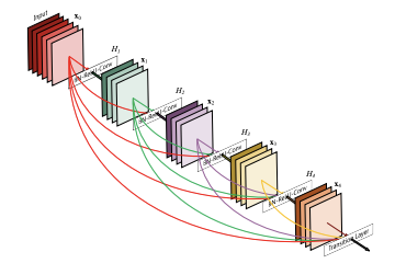
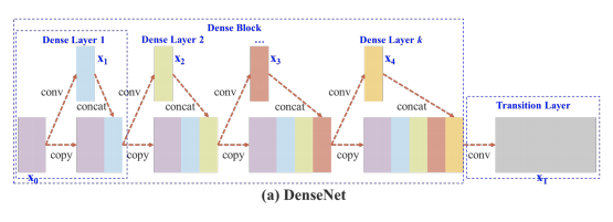
In CSPResNext50 and CSPDarknet53, the DenseNet has been edited to separate the feature map of the base layer by copying it and sending one copy through the dense block and sending another straight on to the next stage. The idea with the CSPResNext50 and CSPDarknet53 is to remove computational bottlenecks in the DenseNet and improve learning by passing on an unedited version of the feature map.
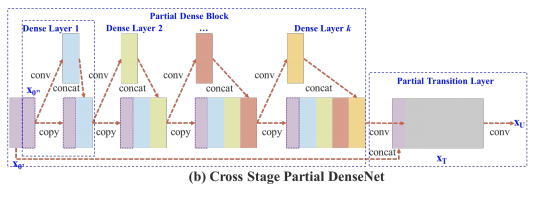
PA-Net Neck
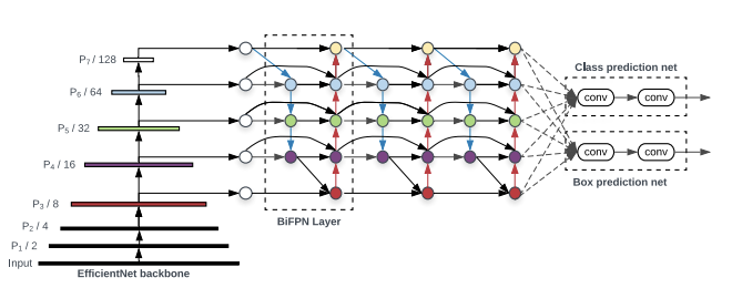
Both YOLOv4 and YOLOv5 implement the PA-NET neck for feature aggregation.
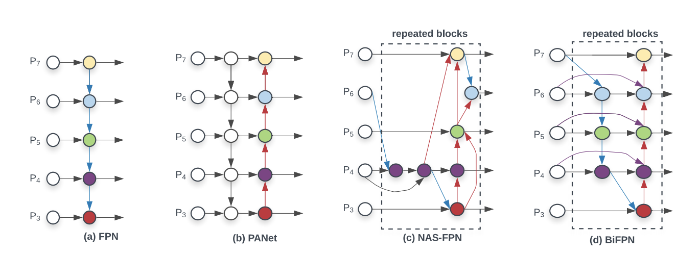
Each one of the P_i above represents a feature layer in the CSP backbone.
The above picture comes from research done by Google Brain on the EfficientDet object detection architecture. The EfficientDet authors found BiFPN to be the best choice for the detection neck, and it is may be an area of further steady for YOLOv4 and YOLOv5 to explore with other implementations here.
It is certainly worth noting here that YOLOv5 borrows research inquiry from YOLOv4 to decide on the best neck for their architecture. YOLOv4 investigated various possibilities for the best YOLO neck including:
- FPN
- PAN
- NAS-FPN
- BiFPN
- ASFF
- SFAM
General Quality of Life Updates for Developer: Why Should I Use YOLOv5?
Compared to other object detection frameworks, YOLOv5 is extremely easy to use for a developer implementing computer vision technologies into an application. I categorize these quality of life updates into the following.
- Easy to install: YOLOv5 only requires the installation of torch and some lightweight python libraries.
- Fast training: The YOLOv5 models train extremely quickly which helps cut down on experimentation costs as you build your model.
- Inference ports that work: You can infer with YOLOv5 on individual images, batch images, video feeds, or webcam ports.
- Intuitive data file system structure: File folder layout is intuitive and easy to navigate while developing
- Easy to apply on mobile devices: You can easily translate YOLOv5 from PyTorch weights to ONXX weights to CoreML to IOS.
Preliminary YOLOv5 Evaluation Metrics
The evaluation metrics presented in this section are preliminary and we can expect a formal research paper to be published on YOLOv5 when the research work is complete and more novel contributions have been made to the family of YOLO models.
That said, it is useful to provide these metrics for a developer who is considering which framework to use today, before the research YOLOv5 papers have been published.
The evaluation metrics below are based on performance on the COCO dataset which contains a wide range of images containing 80 object classes. For more detail on the performance metric, see this post on what is mAP.
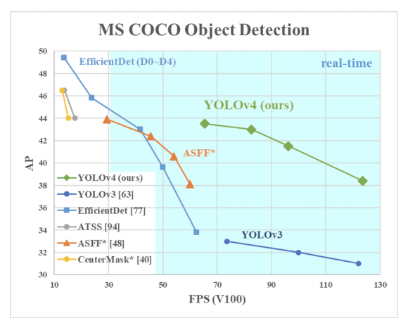
The official YOLOv4 paper publishes the following evaluation metrics running their trained network on the COCO dataset on a V100 GPU:
With the initial release of the first YOLOv5 V1 model, the YOLOv5 repository published the following:
These graphs invert the FPS x-axis vs ms/img, but we can quickly invert the YOLOv5 axis to estimate frame per numbers around 200-300FPS on the same V100 GPU, while achieving higher mAP.
It is also important to note here the new release of YOLOv4-tiny a very small and very performant model in the Darknet Repository.
The evaluation metrics for YOLOv4-tiny read:
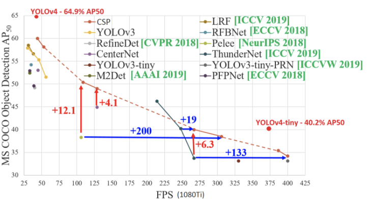
Which means it is very fast and very performant. But the important thing to notice here is that the evaluation metric is AP_50 - which means the average precision at 50% iOU. With this more lenient metric in mind, we must compare against the full table for YOLOv5:
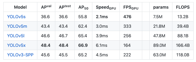
Where we can see that the YOLOv5s (a similar model in speed and model size) achieves 55.8 AP_50.
The comparison is a little more complicated here due to the fact that the YOLOv4-tiny model is evaluated on a 1080Ti which is maximum 2X slower than the V100 used in the YOLOv5 table.
Needless to say, there will be more narrowly matched benchmarks to come and some are underway in this GitHub issue. WongKinYiu, author of the CSP repo above and second author of YOLOv4, provides comparable benchmarks.
From this point of view, YOLOv4 emerges as the superior architecture. It is worth noting however, that in this comparison, YOLOv4 is trained in the Ultralytics YOLOv3 repository (not the native Darknet) including most of the training enhancements in the YOLOv5 repository, showing mAP improvements.
YOLOv5 Labeling Format: YOLOv5 PyTorch TXT
The YOLOv5 PyTorch TXT annotation format is similar to YOLO Darknet TXT but with the addition of a YAML file containing model configuration and class values.
Depending on the annotation tool you use, you'll need to make sure to convert annotations to work with YOLOv5. Roboflow allows you to input 27 different labeling formats and export them to work with YOLOv5. If you uses VOTT, LabelImg, CVAT, or another tool, you can convert those labels to work with YOLOv5.
YOLOv5 Labeling Tool
Ultralytics, the creator of YOLOv5, partners with Robflow as the suggested YOLOv5 labeling tool. You can read more about how Roboflow works with YOLOv5 in the Datasets, Labeling, and Active Learning section of the YOLOv5 Github repo.
Deploy to Roboflow
Once you have finished training a YOLOv5 model, you will have a set of trained weights ready for use with a hosted API endpoint. You can upload your model weights to Roboflow Deploy with the deploy() function in the Roboflow pip package to use your trained weights in the cloud.
To upload model weights, first create a new project on Roboflow, upload your dataset, and create a project version. Check out our complete guide on how to create and set up a project in Roboflow. Then, write a Python script with the following code:
import roboflow

roboflow.login()

rf = roboflow.Roboflow()

project = rf.workspace().project(PROJECT_ID)

project.version(DATASET_VERSION).deploy(model_type=”yolov5”, model_path=f”{HOME}/runs/detect/train/”)
Replace PROJECT_ID with the ID of your project and DATASET_VERSION with the version number associated with your project. Learn how to find your project ID and dataset version number.
Shortly after running the above code, your model will be available for use in the Deploy page on your Roboflow project dashboard.
Deploy Your Model to the Edge
In addition to using the Roboflow hosted API for deployment, you can use Roboflow Inference, an open source inference solution that has powered millions of API calls in production environments. Inference works with CPU and GPU, giving you immediate access to a range of devices, from the NVIDIA Jetson to TRT-compatible devices to ARM CPU devices.
With Roboflow Inference, you can self-host and deploy your model on-device.
You can deploy applications using the Inference Docker containers or the pip package. In this guide, we are going to use the Inference Docker deployment solution. First, install Docker on your device. Then, review the Inference documentation to find the Docker container for your device.
For this guide, we'll use the GPU Docker container:
docker pull roboflow/roboflow-inference-server-gpuThis command will download the Docker container and start the inference server. This server is available at http://localhost:9001. To run inference, we can use the following Python code:
import requests

workspace_id = ""
model_id = ""
image_url = ""
confidence = 0.75
api_key = ""

infer_payload = {
    "image": {
        "type": "url",
        "value": image_url,
    },
    "confidence": confidence,
    "iou_threshold": iou_thresh,
    "api_key": api_key,
}
res = requests.post(
    f"http://localhost:9001/{workspace_id}/{model_id}",
    json=infer_object_detection_payload,
)

predictions = res.json()
Above, set your Roboflow workspace ID, model ID, and API key.
Also, set the URL of an image on which you want to run inference. This can be a local file.
To use your YOLOv5 model commercially with Inference, you will need a Roboflow Enterprise license, through which you gain a pass-through license for using YOLOv5. An enterprise license also grants you access to features like advanced device management, multi-model containers, auto-batch inference, and more.
To learn more about deploying commercial applications with Roboflow Inference, contact the Roboflow sales team.
Conclusion
The initial release of YOLOv5 is very fast, performant, and easy to use. While YOLOv5 has yet to introduce novel model architecture improvements to the family of YOLO models, it introduces a new PyTorch training and deployment framework that improves the state of the art for object detectors. Furthermore, YOLOv5 is very user friendly and comes ready to use on custom objects "out of the box".
Stepping back, it is a great time to be working on computer vision, where the state of the art is advancing so rapidly.
Frequently Asked Questions
What architecture does YOLOv5 use?
YOLOv5 uses a Convolutional Neural Network (CNN) backbone to form image features. These features are combined in the model neck and sent to the head. The model head then interprets the combined features to predict the class of an image.
Is YOLOv5 a single-stage detector?
Yes, the YOLOv5 model is a single-stage detector.