Following this tutorial, you only need to change a couple lines of code to train an object detection model to your own dataset.
Computer vision is revolutionizing medical imaging. Algorithms are helping doctors identify 1 in ten cancer patients they may have missed. There are even early indications that radiological chest scans can aid in COVID-19 identification, which may help determine which patients require lab-based testing. Automated analysis will help us scale up the field of medicine so more patients will be able to get better care for less money.
Update: YOLO v5 has been released
If you're Ok with using PyTorch instead of Tensorflow, we recommend jumping to the YOLOv5 tutorial. You'll have a trained YOLOv5 model on your custom data in minutes.
To that end, in this example we will walkthrough training an object detection model using the TensorFlow object detection API. While this tutorial describes training a model on a microscopy data, it can be easily adapted to any dataset with very few adaptations.
Impatient? Skip directly to the Colab Notebook.
The sections of our example are as follows:
- Introducing our open source computer vision dataset
- Preparing our images and annotations
- Creating TFRecords and Label Maps
- Training Our Model
- Model Inference
Throughout this tutorial, we’ll make use of Roboflow, a tool that dramatically simplifies our data preparation and training process by creating a hosted computer vision pipeline. Roboflow has a free plan, so we’ll be all set for this example.
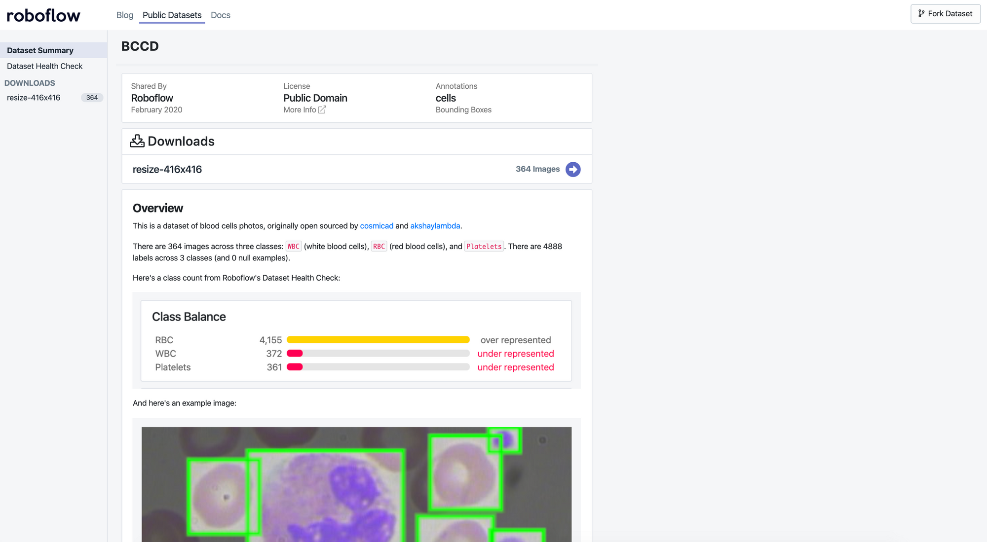
Our Example Dataset: Blood Cell Count and Detection (BCCD)
Our example dataset is 364 images of cell populations and 4888 labels identifying red blood cells, white blood cells, and platelets extracted from microscope slides. Originally open sourced two years ago by comicad and akshaymaba, and available at https://public.roboflow.com. (Note the version hosted on Roboflow includes minor label improvements versus the original release.)
Fortunately, this dataset comes pre-labeled by domain experts, so we can jump right into preparing our images and annotations for our model.
Knowing the presence and ratio of red blood cells, white blood cells, and platelets for patients is key to identifying potential maladies. Enabling doctors to increase their accuracy and throughput of identifying said blood counts can massively improve healthcare for millions.
For your custom data, consider labelling them using tools like Roboflow, LabelImg, CVAT, LabelMe, or VoTT.
Preparing Our Images and Annotations
Going straight from data collection to model training leads to suboptimal results. There may be problems with the data. Even if there aren’t, applying image augmentation expands your dataset and reduces overfitting.
Preparing images for object detection includes, but is not limited to:
- Verifying your annotations are correct (e.g. none of the annotations are out of frame in the images)
- Ensuring the EXIF orientation of your images is correct (i.e. your images are stored on disk differently than how you view them in applications, see more)
- Resizing images and updating image annotations to match the newly sized images
- Checking the health of our dataset, like its class balance, images sizes, and aspect ratios — and determining how these might impact preprocessing and augmentations we want to perform
- Various color corrections that may improve model performance like grayscale and contrast adjustments
Similar to tabular data, cleaning and augmenting image data can improve your ultimate model’s performance more than architectural changes in your model.
Let’s take a look at the “Health Check” of our dataset:
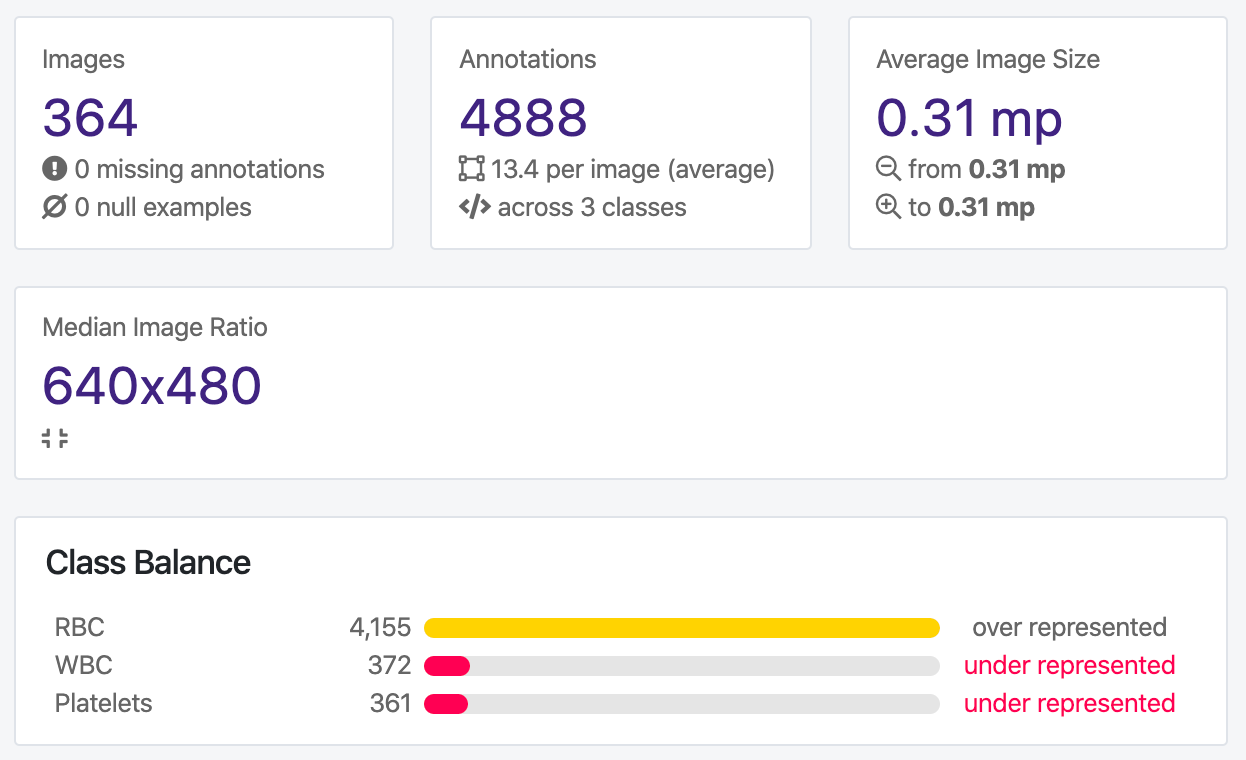
We can clearly see we have a large class imbalance present in our dataset. We have significantly more red blood cells than white blood cells or platelets represented in our dataset, which may cause issues with our model training. Depending on our problem context, we may want to prioritize identification of one class over another as well.
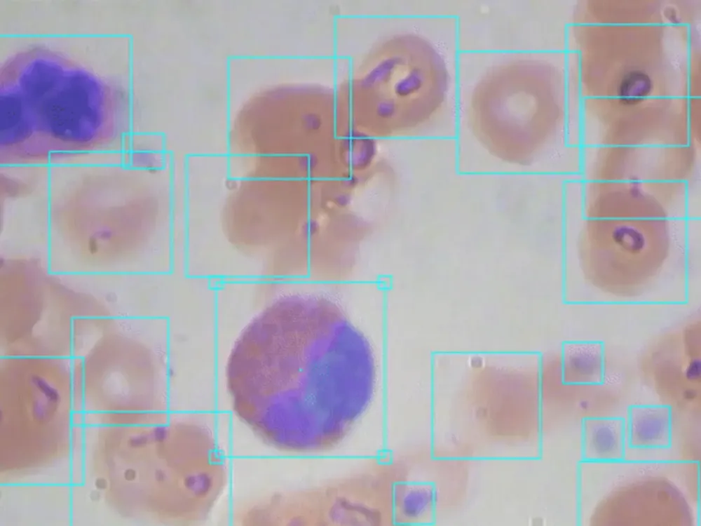
Moreover, we can see from the annotation heat map that our images are all the same size, which makes our resize decision easier.
Annotation heat map using Roboflow
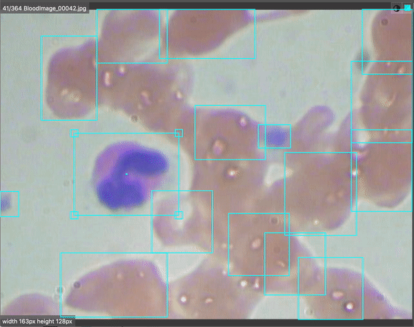
When examining how our objects (cells and platelets) are distributed across our images, we see our red blood cells appear all over, our platelets are somewhat scattered towards the edges, and our white blood cells are clustered in the middle of our images.
Given this, we may want to be weary of cropping the edges of our images when detecting RBC and platelets, but should we just be detecting white blood cells, edges appear less essential. We also want to check that our training dataset is representative of our out-of-sample images. For example, can we expect white blood cells to commonly be centered in newly collected data?
For your custom dataset, upload your images and their annotations to Roboflow following this simple step-by-step guide.
Creating TFRecords and Label Maps
We’ll be using a TensorFlow implementation of Faster R-CNN (more on that in a moment), which means we need to generate TFRecords for TensorFlow to be able to read our images and their labels. TFRecord is a file format that contains both our images and their annotations. It’s serialized at the dataset-level, meaning we create one set of records for our training set, validation set, and testing set. We’ll also need to create a label_map, which maps our label names (RBC, WBC, and platelets) to numbers in a dictionary format.
Frankly, TFRecords are a little cumbersome. As a developer, your time should be focused on fine tuning your model or the business logic of using your model rather than writing redundant code to generate annotation file formats. So, we’ll use Roboflow to generate our TFRecords and label_map files for us with a few clicks.
First, visit the dataset we’ll be using here: https://public.roboflow.ai/object-detection/bccd/1 (Note we’re using a specific version of the dataset. Images have been resized to 416x416.)
Next, click “Download.” You may be prompted to create a free account with email or GitHub.
When downloading, you can download in a variety of formats and download either locally to your machine, or generate a code snippet. For our purposes, we want to generate TFRecord files and create a download code snippet (not download files locally).
Export the dataset
You’ll be given a code snippet to copy. That code snippet contains a link to your source images, their labels, and a label map split into train, validation, and test sets. Hang on to it.
For your custom dataset, if you followed the step-by-step guide from uploading images, you’ll have been prompted to create train, valid, test splits. You’ll also be able to export your dataset to any format you need.
Training Our Model
We’ll be training a Faster R-CNN neural network. Faster R-CNN is a two-stage deep learning object detector: first it identifies regions of interest, and then passes these regions to a convolutional neural network. The outputted features maps are passed to a support vector machine (SVM) for classification. Regression between predicted bounding boxes and ground truth bounding boxes are computed. Faster R-CNN, despite its name, is known as being a slower model than some other choices (like YOLOv4 or MobileNet) for inference but slightly more accurate. For a deeper dive on the machine learning behind it, consider reading this post!
Faster R-CNN is one of the many model architectures that the TensorFlow Object Detection API provides by default, including with pre-trained weights. That means we’ll be able to initiate a model trained on COCO (common objects in context) and adapt it to our use case.
TensorFlow even provides dozens of pre-trained model architectures on the COCO dataset.
We’ll also be taking advantage of Google Colab for our compute, a resource that provides free GPUs. We’ll take advantage of Google Colab for free GPU compute (up to 12 hours).
Our Colab Notebook is here. Also check out the GitHub repository.
You need to be sure to update your code snippet where the cell calls for it with your own Roboflow exported data. Other than that, the notebook trains as-is!
There are a few things to note about this notebook:
- For the sake of running an initial model, the number of training steps is constrained to 10,000. Increase this to improve your results, but be mindful of overfitting!
- The model configuration file with Faster R-CNN includes two types of data augmentation at training time: random crops, and random horizontal and vertical flips.
- The model configuration file default batch size is 12 and the learning rate is 0.0004. Adjust these based on your training results.
- The notebook includes an optional implementation of TensorBoard, which enables us to monitor the training performance of our model in real-time.
In our example of using BCCD, after training for 10,000 steps, we see outputs like the following in TensorBoard:
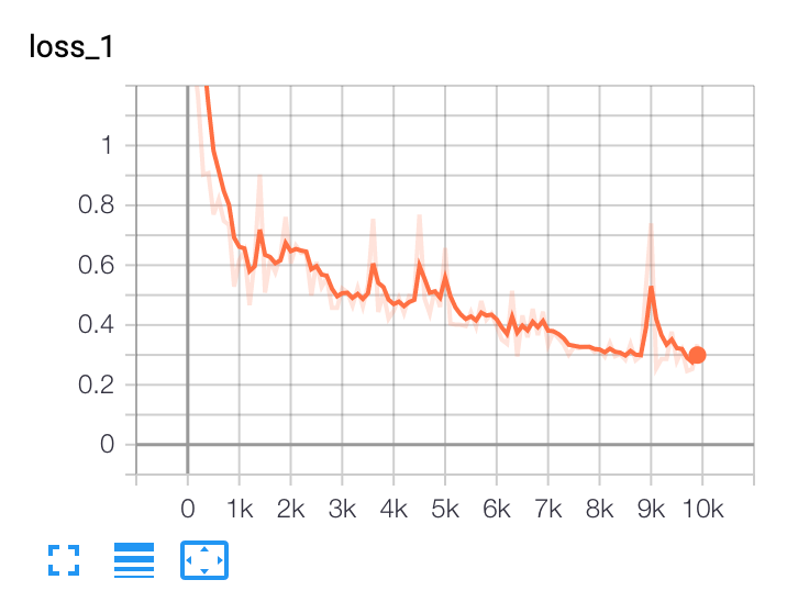
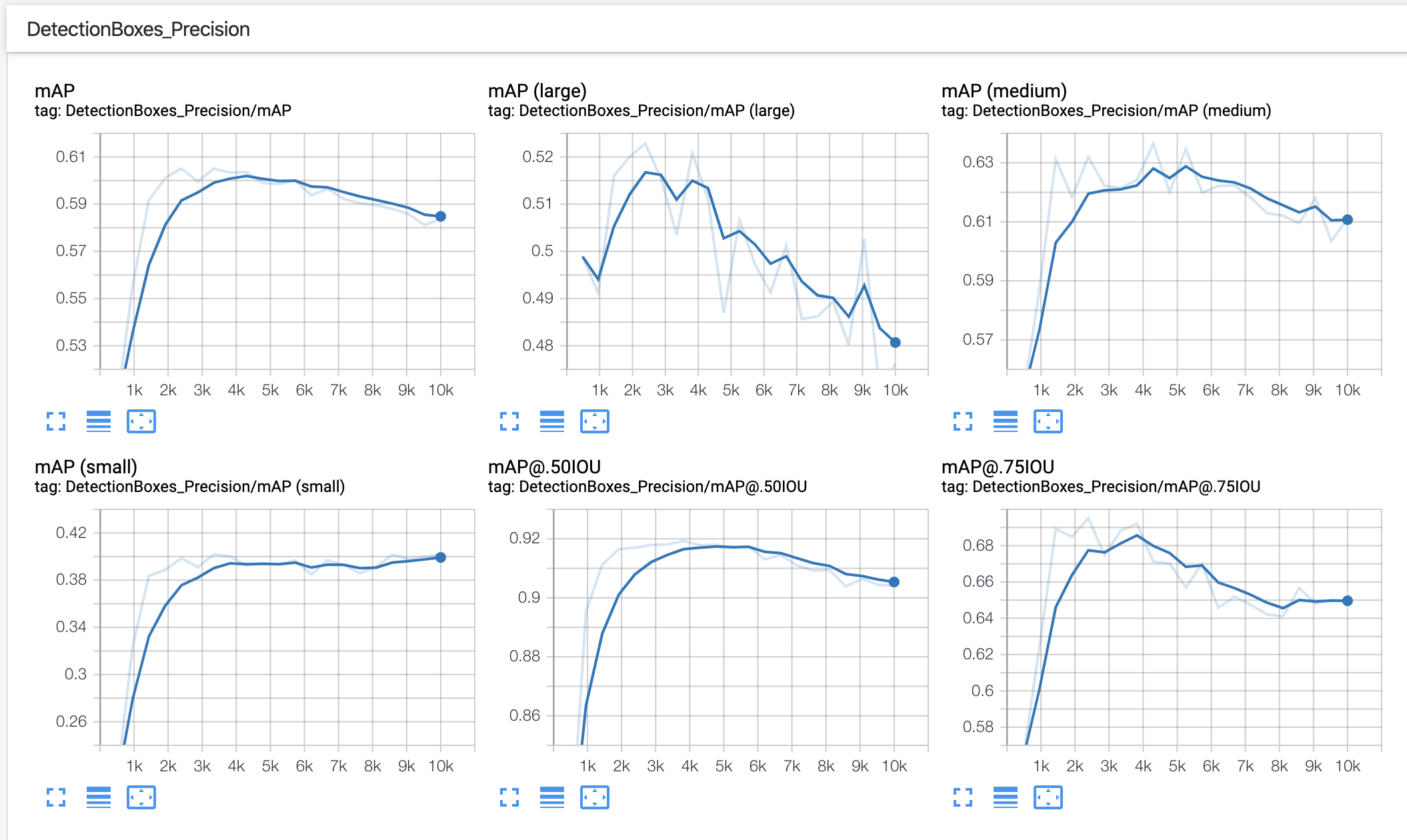
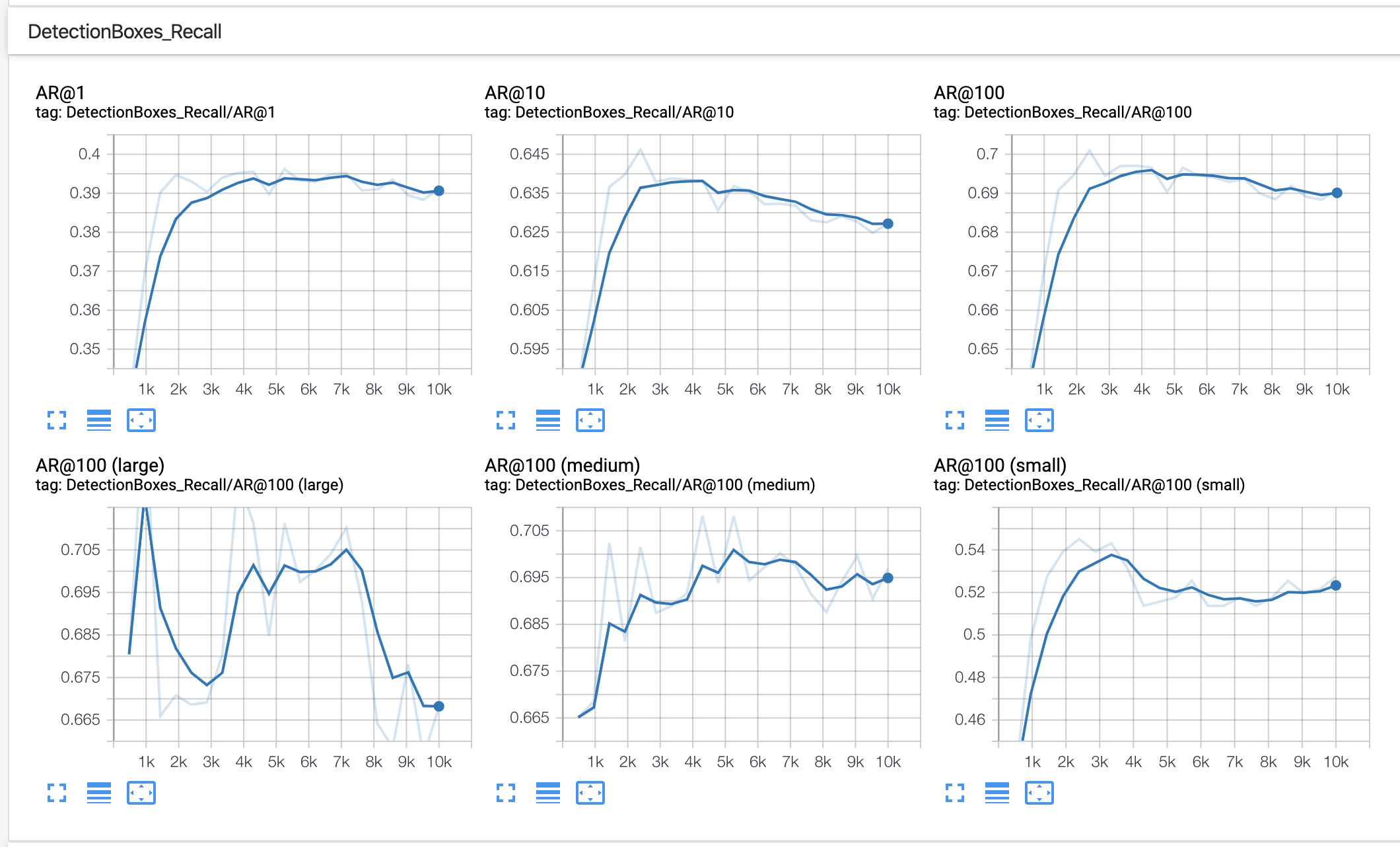
In this example, we should consider collecting or generating more training data and making use of greater data augmentation.
For your custom dataset, these steps will be largely identical as long as you update your Roboflow export link to be specific to your dataset. Keep an eye on your TensorBoard outputs for overfitting.
Model Inference
As we train our Faster R-CNN model, its fit is stored in a directory called ./fine_tuned_model. There are steps in our notebook to save this model fit — either locally downloaded to our machine, or via connecting to our Google Drive and saving the model fit there. Saving the fit of our model not only allows us to use it later in production, but we could even resume training from where we left off by loading the most recent model weights!
In this specific notebook, we need to add raw images to the /data/test directory. It contains TFRecord files, but we want raw (unlabeled) images for our model to make predictions.
We should upload test images that our model hasn’t seen. To do so, we can download the raw test images from Roboflow to our local machines, and add those images to our Colab Notebook.
Revisit our dataset download page.
Click download. For format, select COCO JSON and download locally to your own computer. (You can actually download any format that isn’t TFRecord to get raw images separate from annotation formats!)
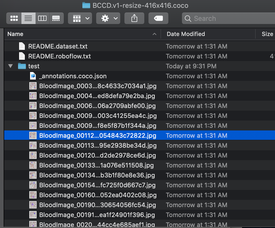
Once unzipping this file locally, you’ll see the test directory raw images:
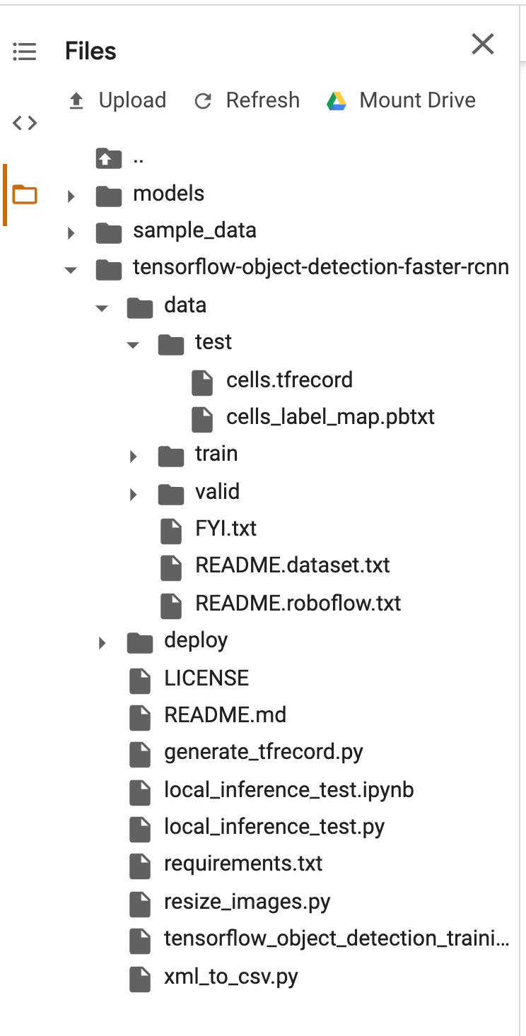
Now, in the Colab notebook, expand the left hand panel to show the test folder:
Right click on the “test” folder and select “Upload.” Now, you can select all the images from your local machine that you just downloaded!
Inside the notebook, the remainder of the cells go through how to load the saved, trained model we created and run them on the images you just uploaded.
For BCCD, our output looks like the following:
Our model does pretty well after 10,000 epochs
For your custom dataset, this process looks very similar. Instead of downloading images from BCCD, you’ll download images from your own dataset, and re-upload them accordingly.
Next Steps with your Trained Object Detection Model
You’ve trained an object detection model to a custom dataset.
Now, making use of this model in production begs the question of identifying what your production environment will be. For example, will you be running the model in a mobile app, via a remote server, or even on a Raspberry Pi? How you’ll use your model determines the best way to save and convert its format.
Consider these resources as next steps based on your problem: converting to TFLite (for Android and iPhone), converting to CoreML (for iPhone apps), converting for use on a remote server, or deploying to a Raspberry Pi.
Build and deploy with Roboflow for free
Use Roboflow to manage datasets, train models in one-click, and deploy to web, mobile, or the edge. With a few images, you can train a working computer vision model in an afternoon.