This is a lightly edited guest post by Roboflow user Shayan Ali Bhatti, who used Roboflow to train an object detection model to identify items in grocery stores.
Reposted with permission. Original content here.
In this article, I present an application of the latest version of popular deep learning algorithm YOLO i.e. YOLOv5, to detect items present in a retail store shelf. This application can be used to keep track of inventory of items simply using images of the items on shelf.

Introduction
Object detection is a computer vision task that requires object(s) to be detected, localized and classified. In this task, first we need our machine learning model to tell if any object of interest is present in the image.
If present, then draw a bounding box around the object(s) present in the image. In the end, the model must classify the object represented by the bounding box. This task requires fast object detection so that it can be implemented in real-time. One of its major applications is its use in real-time object detection in self-driving vehicles.
Joseph Redmon, et al. originally designed YOLOv1, v2 and v3 models that perform real-time object detection. YOLO “You Only Look Once” is a state-of-the-art real-time deep learning algorithm used for object detection, localization and classification in images and videos. This algorithm is very fast, accurate and at the forefront of object detection based projects.
Each of the versions of YOLO kept improving the previous in accuracy and performance. Then came YOLOv4 developed by another team, further adding to performance of model and finally the YOLOv5 model was introduced by Glenn Jocher in June 2020.
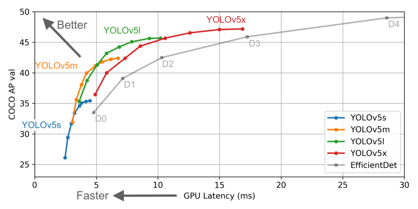
This model significantly reduces the model size (YOLOv4 on Darknet had 244MB size whereas YOLOv5 smallest model is of 27MB). YOLOv5 also claims a faster accuracy and more frames per second than YOLOv4 as shown in graph below, taken from Roboflow’s website.
More details about how YOLO works can be found on internet. In this article, I will only focus on the use of YOLOv5 for retail item detection.
Objective
To use YOLOv5 to draw bounding boxes over retail products in pictures using SKU110k dataset.

Dataset
To do this task, first I downloaded the SKU110k image dataset from the following link:
http://trax-geometry.s3.amazonaws.com/cvpr_challenge/SKU110K_fixed.tar.gz
The SKU110k dataset is based on images of retail objects in a densely packed setting. It provides training, validation and test set images and the corresponding .csv files which contain information for bounding box locations of all objects in those images. The .csv files have object bounding box information written in the following columns:
image_name,x1,y1,x2,y2,class,image_width,image_height
where x1,y1 are top left co-ordinates of bounding box and x2,y2 are bottom right co-ordinates of bounding box, rest of parameters are self-explanatory. An example of parameters of train_0.jpg image for one bounding box, is shown below. There are several bounding boxes for each image, one box for each object.
train_0.jpg, 208, 537, 422, 814, object, 3024, 3024
In the SKU110k dataset, we have 2940 images in the test set, 8232 images in the train set and 587 images in the validation set. Each image can have varying number of objects, hence, varying number of bounding boxes.
Label and Annotate Data with Roboflow for free
Use Roboflow to manage datasets, label data, and convert to 26+ formats for using different models. Roboflow is free up to 10,000 images, cloud-based, and easy for teams.
Methodology
From the dataset, I took only 998 images from the training set and went to the Roboflow website which provides online image annotation service in different formats including YOLOv5 supported format. The reason for picking only 998 images from training set is that Roboflow’s dataset management service is only free for the first 1000 images.
Preprocessing
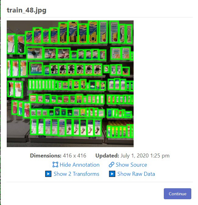
Preprocessing of images includes resizing them to 416x416x3. This is done on Roboflow’s platform. An annotated, resized image is shown in figure below:
Automatic Annotation
On Roboflow's website, the bounding box annotation .csv file and images from training set are uploaded and Roboflow’s computer vision ETL service automatically draws bounding boxes on images using the annotations provided in the .csv files as shown in image above.
Data Generation
Roboflow also gives option to generate a dataset based on user defined split. I used 70–20–10 training-validation-test set split. After the data is generated on Roboflow, we get the original images as well as all bounding box locations for all annotated objects in a separate text file for each image, which is convenient.
Finally, we get a link to download the generated data with label files. This link contains a key that is restricted to only your account and is not supposed to be shared.
Hardware Used
The model was trained on Google Colab Pro notebook with Tesla P100 16GB Graphics Card. It costs $9.99 and it is good for a month’s use. Google Colab notebook can also be used which is free but usage session time is limited.
Code
I recommend using the YOLOv5 Google Colab notebook provided by Roboflow.
It is originally trained for COCO dataset but can be tweaked for custom tasks which is what I did. I started by cloning YOLOv5 and installing the dependencies mentioned in requirements.txt file. Also, the model is built for Pytorch, so I import that.
!git clone https://github.com/ultralytics/yolov5  # clone repo
!pip install -r yolov5/requirements.txt  # install dependencies
%cd yolov5

import torch
from IPython.display import Image, clear_output  # to display images
from utils.google_utils import gdrive_download  # to download models/datasets

clear_output()
print('Setup complete. Using torch %s %s' % (torch.__version__, torch.cuda.get_device_properties(0) if torch.cuda.is_available() else 'CPU'))
Next, I download the dataset that I created at Roboflow.com. The following code will download training, test and validation set and annotations too. It also creates a .yaml file which contains paths for training and validation set as well as what classes are present in our data.
# Export code snippet and paste here%cd /content!curl -L "https://app.roboflow.ai/ds/dNpgZfRlr4?key=REDACTED" > roboflow.zip; unzip roboflow.zip; rm roboflow.zip
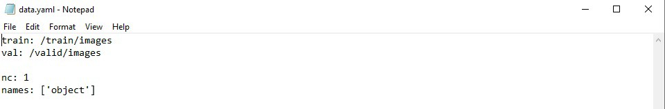
This file tells the model the location path of training and validation set images along with the number of classes and the names of classes. For this task, number of classes is “1” and the name of class is “object” as we are only looking to predict bounding boxes. data.yaml file can be seen below:
Network Architecture
Next let’s define the network architecture for YOLOv5. It is the same architecture used by the author Glenn Jocher for training on COCO dataset. I didn't change anything in the network. However, few tweaks were needed to change bounding box size, color and also to remove labels otherwise labels would jumble the image because of so many boxes. These tweaks were made in detect.py and utils.py file. The network is saved as custom_yolov5.yaml file
%cd /content/
##write custom model .yaml
#you can configure this based on other YOLOv5 models in the models directory
with open('yolov5/models/custom_yolov5s.yaml', 'w') as f:
  # parameters
  f.write('nc: ' + num_classes + '\n')
  #f.write('nc: ' + str(len(class_labels)) + '\n')
  f.write('depth_multiple: 0.33'  + '\n') # model depth multiple
  f.write('width_multiple: 0.50'  + '\n')  # layer channel multiple
  f.write('\n')
  f.write('anchors:' + '\n')
  f.write('  - [10,13, 16,30, 33,23] ' + '\n')
  f.write('  - [30,61, 62,45, 59,119]' + '\n')
  f.write('  - [116,90, 156,198, 373,326] ' + '\n')
  f.write('\n')

  f.write('backbone:' + '\n')
  f.write('  [[-1, 1, Focus, [64, 3]],' + '\n')
  f.write('   [-1, 1, Conv, [128, 3, 2]],' + '\n')
  f.write('   [-1, 3, Bottleneck, [128]],' + '\n')
  f.write('   [-1, 1, Conv, [256, 3, 2]],' + '\n')
  f.write('   [-1, 9, BottleneckCSP, [256]],' + '\n')
  f.write('   [-1, 1, Conv, [512, 3, 2]], ' + '\n')
  f.write('   [-1, 9, BottleneckCSP, [512]],' + '\n')
  f.write('   [-1, 1, Conv, [1024, 3, 2]],' + '\n')
  f.write('   [-1, 1, SPP, [1024, [5, 9, 13]]],' + '\n')
  f.write('   [-1, 6, BottleneckCSP, [1024]],' + '\n')
  f.write('  ]' + '\n')
  f.write('\n')

  f.write('head:'  + '\n')
  f.write('  [[-1, 3, BottleneckCSP, [1024, False]],'  + '\n')
  f.write('   [-1, 1, nn.Conv2d, [na * (nc + 5), 1, 1, 0]],' + '\n')
  f.write('   [-2, 1, nn.Upsample, [None, 2, "nearest"]],' + '\n')

  f.write('   [[-1, 6], 1, Concat, [1]],' + '\n')
  f.write('   [-1, 1, Conv, [512, 1, 1]],' + '\n')
  f.write('   [-1, 3, BottleneckCSP, [512, False]],' + '\n')
  f.write('   [-1, 1, nn.Conv2d, [na * (nc + 5), 1, 1, 0]],' + '\n')

  f.write('   [-2, 1, nn.Upsample, [None, 2, "nearest"]],' + '\n')
  f.write('   [[-1, 4], 1, Concat, [1]],' + '\n')
  f.write('   [-1, 1, Conv, [256, 1, 1]],' + '\n')
  f.write('   [-1, 3, BottleneckCSP, [256, False]],' + '\n')
  f.write('   [-1, 1, nn.Conv2d, [na * (nc + 5), 1, 1, 0]],' + '\n')
  f.write('\n' )
  f.write('   [[], 1, Detect, [nc, anchors]],' + '\n')
  f.write('  ]' + '\n')

print('custom model config written!')
Training
Now I start the training process. I defined the image size (img) to be 416x416, batch size 32 and the model is run for 300 epochs. If we dont define weights, they are initialized randomly.
# train yolov5s on custom data for 300 epochs
%cd /content/yolov5/
!python train.py --img 416 --batch 32 --epochs 300 --data '../data.yaml' --cfg ./models/custom_yolov5s.yaml --weights '' --name yolov5s_results --nosave --cache
It took 4 hours 37 minutes for training to complete on a Tesla P100 16GB GPU provided by Google Colab Pro. After the training is complete, model’s weights are saved in Google drive as last_yolov5_results.pt
from google.colab import drive
drive.mount('/content/gdrive',force_remount=True)
%cp /content/yolov5/weights/last_yolov5s_results.pt /content/gdrive/My\ Drive
Observations
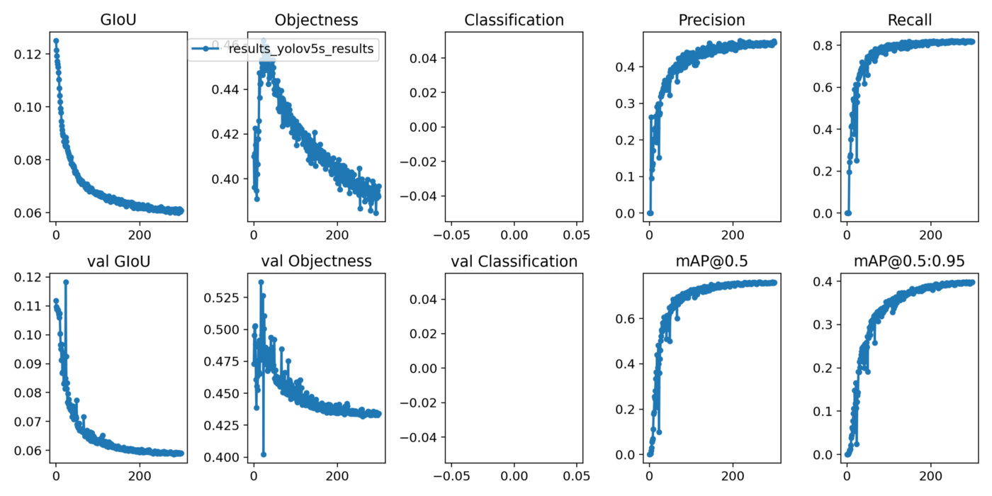
We can visualize important evaluation metrics after the model has been trained using the following code:
# we can also output some older school graphs if the tensor board isn't working for whatever reason...
from utils.utils import plot_results; plot_results()  # plot results.txt as results.png
Image(filename='./results.png', width=1000)  # view results.png
The following 3 parameters are commonly used for object detection tasks:
· GIoU is the Generalized Intersection over Union which tells how close to the ground truth our bounding box is.
· Objectness shows the probability that an object exists in an image. Here it is used as loss function.
· mAP is the mean Average Precision telling how correct are our bounding box predictions on average. It is area under curve of precision-recall curve.
It is seen that Generalized Intersection over Union (GIoU) loss and objectness loss decrease both for training and validation. Mean Average Precision (mAP) however is at 0.7 for bounding box IoU threshold of 0.5. Recall stands at 0.8 as shown below:
Now comes the part where we check how our model is doing on test set images using the following code:
# when we ran this, we saw .007 second inference time. That is 140 FPS on a TESLA P100!
%cd /content/yolov5/
!python detect.py --weights weights/last_yolov5s_results.pt --img 416 --conf 0.4 --source ../test/images
Results
Following images show the result of our YOLOv5 algorithm trained to draw bounding boxes on objects. The results are pretty good.
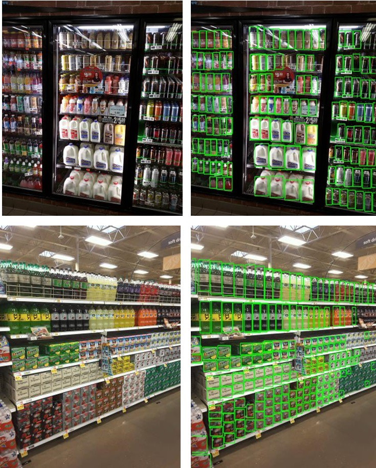
The inference time was just 0.009 seconds and the weights file turned out to be just 13.9MB.
Link To Repository
Following link contains the repository for the project. Please make sure you copy the code from jupyter notebook in Google Colab as it was originally written there.
https://github.com/shayanalibhatti/Retail-Store-Item-Detection-using-YOLOv5
The utils.py and detect.py files in the repository are tweaked to remove object labels and make green thin bounding boxes.
Conclusion
Naming controversies aside, YOLOv5 performs well and can be customized to suit our needs. However, training the model can take significant GPU power and time. It is recommended to use at least Google Colab with 16GB GPU or preferably a TPU to speed up the process for training the large dataset.
This retail object detector application can be used to keep track of store shelf inventory or for a smart store concept where people pick stuff and get automatically charged for it. YOLOv5’s small weight size and good frame rate will pave its way to be first choice for embedded-system based real-time object detection tasks. Try YOLOv5 on your own dataset.